Prerequisites: Basic probability and matrices knowledge
First introduced by Andrey Markov (a Russian mathematician), Markov chains are one of the most important stochastic processes used in this day and age. Used for predicting the weather, forecasting market trends and even used in Google’s own PageRank algorithm (used to rank webpages based on search results), Markov chains have proved to be a very useful mathematical tool.
What is a Markov chain?
A Markov Chain is a type of stochastic process that satisfies the Markov property, which is where the past and future are independent when the present is known. In other words, if the current state of the process is known, then no additional information regarding its past states is required to make predictions about its future states (Myers, Wallin and Wikström, 2017). In simple terms: The probability of a certain “change of state” is independent of what had happened previously.
In more formal, mathematical terms, the definition of a Markov Chain can be expressed as follows:
A sequence of random variables X0 , X1 , X2 , … taking values in the state space {1, 2, … , M} is called a Markov chain if for all n >= 0
P(Xn+1 = j | Xn = i, Xn-1 = in-1, … , X0 = i0 ) = P(Xn+1 = j | Xn = i)n
(Blitzstein 2018).
Breaking down the definition above, n here is the index of the process and represents the evolution of the process over time. The set of possible values Xn (a random variable) can take is called the state space, a finite set of numbers which is usually {1, 2, … , M}. i and j represent states in our stochastic process, therefore P(Xn+1 = j | Xn = i) represents the probability that the next state will be j given that the current state is i. This is also known as the transition probability from state i to state j (Blitzstein 2018).
In a nutshell, the mathematical definition states that for a process to be a Markov Chain, only the most recent state in our process (i.e. Xn) matters for predicting our next state (i.e. Xn+1) and all other states before Xn can be ignored to find our probability.
Markov processes
Below are examples of two different processes – one that holds the Markov property, and another that does not.
Process 1: There is an urn with exactly 50 red balls and 50 blue balls inside. Every minute, a person randomly takes out a certain ball from the urn without replacement (i.e. the ball is not put back into the urn). This process does not hold a Markov property, as the probability of picking out a certain coloured ball changes every time a ball is taken out – probabilities are dependent on all past results. Therefore, we cannot use a Markov chain to predict the probability of outcomes in this process.
Process 2: A city somewhere in the world can only experience two types of weather – sunny and rainy. The probabilities of the weather changing (e.g. sunny to rainy, rainy to sunny) and the probabilities of the weather staying the same (e.g. sunny to sunny, rainy to rainy) are all fixed. This process does hold the Markov property, as the probability of the weather changing or staying the same does not rely on previous data about the weather (e.g. we do not need to know how many days it has been raining previously to predict whether tomorrow will be a rainy day). We can therefore use a Markov chain to predict the probability of outcomes in this process.
Predicting the weather
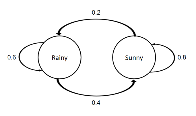
Continuing from the above example, if the city’s weather is currently sunny, there is a 20% chance it rains the next day (and an 80% chance it remains sunny). If the city’s weather is currently rainy, there is a 40% chance it is sunny the next day (and a 60% chance it remains rainy).
Questions:
Q1. Assuming the city is sunny today, what is the probability that it still sunny in 2 days?
Q2. Again, assuming the city is sunny today, what is the probability that it is rainy in 20 days?
Q3. If we do not know what the weather is today and if it were to be decided completely randomly with a 50-50 chance, what is the probability that it is rainy in 5 days?
Solutions:
A1. To start, we could represent the given probabilities in a state diagram as shown below
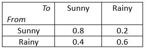
We could also put the probabilities into a table like the following:
Now, to answer the first question of this example, an obvious approach would to be use a tree diagram as follows
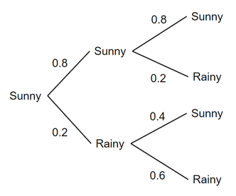
P(Day 2 = Sunny | Today is sunny) = 0.8*0.8 + 0.2*0.4
= 0.64 + 0.08
= 0.72
However, this can be extremely inefficient – especially with questions 2 and 3. Imagine how many trees and calculations that would have to be done in order to get the day 20 probability (we would need to draw 2097150 branches on our tree! This doesn’t include the work of doing the actual calculations either). Instead, we could use a Markov Chain to perform these calculations.
Step 1: Construct the transition matrix
We first need to construct a transition matrix to start the Markov Chain. The transition matrix is a square matrix used to describe the probability transitions of a Markov Chain. Each entry in the matrix contains a non-negative, real number that represents a probability. Each individual row in the transition matrix should add up to 1 (Blitzstein 2018).
In mathematical terms, the definition of transition matrix can be expressed as follows:
Let X0 , X1 , X2 , … be a Markov chain with state space {1, 2, … , M}, and let qij = P(Xn+1 = j | Xn = i) be the transition probability from state i to state j. The M*M matrix Q = (qij) is called the transition matrix of the chain.
(Blitzstein 2018).
In a nutshell, the mathematical definition states that the transition matrix of a Markov chain is a matrix with size M*M, where M is the number of states in the process and the matrix is filled with all transition probabilities.
This is where our table we made earlier come in handy. We can put all the values from the table into a 2*2 matrix to form out transition matrix Q.

The matrix can be read and understood like this:
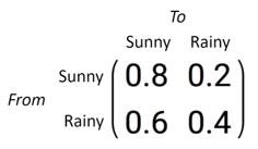
e.g. the probability that the weather goes from sunny to rainy = 0.8
Or in general: the probability that the weather goes from <row> to <column> = <number in pre-specified row and column>
Step 2: Determine the initial conditions
Now, we need to construct a vector that hold our initial conditions. In the case of Q1, we start on a sunny day. We can create a row vector t that represents this.

The vector can be read and understood like this:

Since we know for a fact that today is a sunny day, the probability we start the process on a sunny day is 1 (and a probability of 0 that we start the process on a rainy day).
Step 3: Vector and matrix multiplication
We now have all the items we need to calculate the probability that it is rainy in 2 days. We can calculate this value by setting the matrix to the power of the number of days (in this case 2) and then multiplying the row vector with the exponent matrix. Below are the calculations used to answer Q1

We get a row vector as our solution, which can be interpreted like this (the sum of all values in the final vector should add up to 1)

So, our answer to Q1 would be the first column of our row vector, which is 0.72, the same answer we got from out probability tree calculation! P(Day 2 = Sunny | Today is sunny) = 0.72
A2. Same method as A1, but now we set the exponent of the matrix to 20 (for 20 days)

A3. Since we do not know what today’s weather is, we will change the initial conditions in our vector

Probability that today is a sunny day and probability that today a rainy day are now both equal. We can now use our usual method, setting the exponent of the matrix to 5

Forecasting market trends
Now to another, slightly harder example where Markov Chains are used very often – forecasting stock market trends. Using Markov Chains, we can calculate the likelihood of future market trends, based on the market’s current state. There are 3 primary market trends:
- Bullish: Prices of stocks tend to rise – upward trend in prices
- Bearish: Prices of stocks tend to fall – downward trend in prices
- Stagnant: Prices of stocks tend to remain constant – prices do not move upward nor downward in trend
Using technical analysis on historical financial data, it is possible to find patterns within the markets, which can be used to estimate probabilities of market trend shifts (Myers, Wallin and Wikström, 2017). However, for simplicity, the following values used in the example are not based on real data – they were merely random numbers created for this example. With that in mind, please do not use the following data for any financial activities.
Let’s now consider the market for Stock A. Stock A’s market exhibits Markov properties with the following patterns: After a week of a bullish market, there is a 10% chance the market goes bearish and a 25% chance the market goes stagnant. After a week of a bearish market, there is a 20% chance the market goes stagnant and a 5% chance the market goes bullish. Finally, after a week of a stagnant market, there is a 45% chance the market goes bearish and a 45% chance the market goes bullish.
Questions (feel free to attempt these before looking at the solutions):
Q1. Assuming this week’s market was bullish, what is the probability that the market goes bearish in 3 weeks?
Q2. We do not know the market condition this week. However, we do know that there is a 40% chance this week’s market is bearish and a 60% chance this week’s market is bullish. What is the probability that the market is stagnant in 5 weeks?
Q3. Again, we do not know the market condition this week. This time, the market has an equal chance/probability of starting out in any one of the three trends. If we were to wait for the market for an extremely long time (say an infinite number of weeks), what is the approximate probability that the market will be bullish?
Solutions:
A1. To start, lets draw our table of probabilities and state diagram
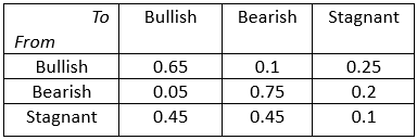
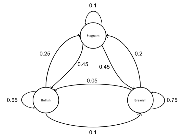
We can now start making our Markov chain
Step 1: Construct the transition matrix
Just like the last example, since we created a table, we can immediately put our values from the table into a matrix

Step 2: Determine the initial conditions
Same thing like last time: let’s construct a row vector with our initial condition – market starts bullish. Remember to make sure the vector columns correspond to what the matrix columns represent!

Step 3: Vector and matrix multiplication
We now have all the items we need to calculate the probability that the market is bearish in 3 weeks. Just like the last example, we set the matrix to the power of the number of weeks (in this case 3) and then multiplying the row vector with the exponent matrix.

A2. First, let’s initialise our row vector with the new initial conditions: A 40% chance this week’s market is bearish and a 60% chance this week’s market is bullish

We can now use our usual method, setting the exponent of the matrix to 5

A3. This question may seem confusing at its surface, but in reality, all that its asking is you to do is to get the probabilities as the number of weeks tends toward infinity (i.e. to set the exponent of Q to an extremely large number)
Let’s initialise our row vector with the new initial conditions: An equal chance of starting with any of the 3 market trends

Now observe the values of our final row vector as we increase the number of weeks
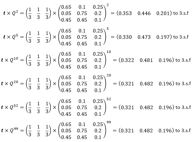
We can see the final vector’s values converge toward (0.321 0.482 0.196). We can also observe that as the exponent of Q gets larger, the final vector tends toward (0.321 0.482 0.196). Therefore, we can say as the number of weeks tends toward infinity, our final vector value tends toward (0.321 0.482 0.196), and the probability the market is bullish tends toward 0.321.
In conclusion, as the number of weeks tends towards infinity (or gets extremely large):
P(Week infinity = bullish) = 0.321 to 3.s.f
Conclusion
Markov chains are an extremely useful tool in the real world, whether it’s predicting the weather, forecasting market trends or simply predicting any process where probabilities are fixed and past events/states do not matter.
Glossary
Markov Chain – A type of stochastic process that satisfies the Markov property.
Stochastic process – A type of process that evolves in a random way e.g. A sequence of random variables changing over time (Blitzstein 2018).
Markov property – If the current state of the process is known, then no additional information regarding its past states is required to make predictions about its future states (Myers, Wallin and Wikström, 2017).
Transition probability – Probability that one state moves to another state e.g. probability that state A changes to state B in one week’s time (Blitzstein 2018).
Transition matrix – A square matrix used to describe the probability transitions of a Markov Chain (Blitzstein 2018).
References
Blitzstein, J.K. (2018) Unit 7: Markov Chains, STAT110x: Introduction to probability. [online] Available at: https://www.edx.org/learn/probability/harvard-university-introduction-to-probability [Accessed 15 Jul. 2024].
Myers, D.S., Wallin, L. and Wikström, P. (2017). An introduction to Markov chains and their applications within finance. [online] Available at: https://www.math.chalmers.se/Stat/Grundutb/CTH/mve220/1617/redingprojects16-17/IntroMarkovChainsandApplications.pdf [Accessed 30 Jul. 2024].

